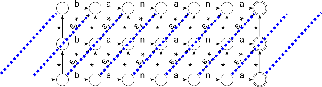
A Levenshtein Automaton is a finite state machine that recognizes all strings within a given edit distance from a fixed string. Here’s a Levenshtein Automaton that accepts all strings within edit distance 2 from “banana”:

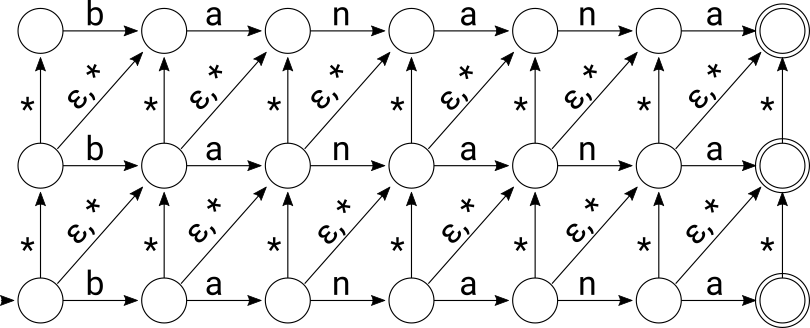
The epsilon transitions represent the empty string. The * transitions are shorthand for “any character” to save space in the diagram, but the actual automaton has one transition for every possible input character anywhere you see a *. The automaton accepts a string s exactly when there’s a directed path from the start state on the lower left to any of the accept states on the right such that the concatenation of all of the labels on the path in order equals s.

The automaton above is an NFA but it looks like three copies of a DFA accepting the string “banana” stacked on top of each other. Transitions between the three DFAs represent edit operations under the Damerau-Levenshtein metric: a transition going up represents the insertion of a character, a diagonal epsilon transition represents the deletion of a character, and a diagonal * transition represents a substitution.

Levenshtein Automata can be used as one part of a data structure that generates spelling corrections. The other component is a Trie that contains all correctly spelled words. Any word that’s accepted by both the Trie and the Levenshtein Automaton is a word that’s correctly spelled and up to edit distance d from the query. Given a query, you’d generate a Levenshtein Automaton for that query with the desired edit distance and then traverse both the automaton and the Trie in parallel, yielding a word whenever you reach an accept state in the Levenshtein Automaton and at a leaf node in the Trie at the same time.

Generating a non-deterministic Levenshtein Automaton is straightforward. The node and edge structure of the automaton above for the query “banana” isn’t a function of the word “banana” at all – only the transition labels would be different if you wanted to create a similar automaton accepting anything within edit distance 2 of any other six-letter word. Increasing or decreasing the edit distance just involves adding or removing one or more rows of identical states. Increasing or decreasing the length of the fixed word just involves adding or removing one or more columns.

Unfortunately, even though generating a non-deterministic Levenshtein Automaton is easy, simulating it efficiently isn’t. In general, simulating all execution paths of an NFA with n states on an input of length m can take time O(nm) just to keep up with the bookkeeping: a state in the simulation is a subset of states in the NFA and you have to update that set of up to n states m times during the simulation.

Schulz and Mihov introduced Levenshtein Automata and showed how to generate and simulate them in linear time in the length of an input string. The implementation they describe involves a preprocessing step that creates a DFA defined by a transition table whose size grows very quickly with the edit distance d. The implementation starts with a two-dimensional table from which many of the entries can be removed because they represent dead states. For d=1, a 5 x 8 table is reduced to just 9 entries, for d=2, a 30 x 32 table is reduced to one with just 80 entries. For d=3 and 4, the tables start with 196 x 128 = 25,088 and 1352 x 512 = 692,224 entries, respectively, before removing dead states.

The Lucene project implemented Schulz and Mihov’s scheme, but only for d = 1 and d = 2. Their implementation uses a Python script from another project, Moman, to generate Java code with the transition tables offline.

It’s hard to beat a table-driven DFA for matching regular expressions, but on the other hand, it’s not clear that the simulation of the Levenshtein Automaton is the bottleneck in a spelling corrector. The size of the Levenshtein Automaton is dwarfed by the size of the Trie containing the correctly spelled words, and since query processing involves simulating both the Trie and the Levenshtein Automaton in parallel, the main bottleneck in the simulation will likely be the I/O expense of loading nodes for the Trie. Because of their high and irregular branching factor, Tries are all but impossible to lay out in memory with any kind of locality of reference for an arbitrary query.

So maybe there’s a simpler way to simulate Levenshtein Automata that’s theoretically slower but will give us about the same real-world performance. Jules Jacobs recently wrote a post describing a pretty substantial simplification that simulates an automaton using states based on rows in the two-dimensional matrix of the Wagner-Fischer algorithm to compute edit distance. The simulation takes O(nd) time for an input of length n, which is essentially as good as an implementation based on Schulz and Mihov’s scheme since d is often small and fixed.

You can also derive an O(nd) time simulation by just directly simulating the NFA that I described at the beginning of this post. You just need to make a few optimizations based on the highly regular structure of this family of NFAs, but all of the optimizations are relatively straightforward. I’ll describe those optimizations in this post. I’ve also implemented everything I describe here in a Go package called levtrie that provides a map-like interface to a Trie equipped with a Levenshtein Automaton.

Alternatives to Levenshtein Automata

First, some more background. You can skip this section and the next if you already understand why Levenshtein Automata are a good choice for indexing a set of words by edit distance.

Edit distance is a metric and there are many data structures that index keys by distance under various metrics. Maybe the most appropriate metric tree for edit distance is the BK-Tree. The BK-Tree, like other metric trees, has two big disadvantages: first, the layout of the tree is highly dependent on the distribution and the insertion order, so it’s hard to quote good bounds on how balanced the tree is in general. Second, during lookups, you have to compute the distance function at each node along the search path, which can be expensive for an metric like edit distance that takes quadratic time to compute (or O(nd) if you optimize for computing distance at most d).

Locality-sensitive hashing is another option, but, like metric trees, even after hashing to a bucket you’re left with a set of candidates on which you need to exhaustively calculate edit distance. It’s also very difficult with most metrics to get anywhere close to perfect recall with locality-sensitve hashing and perfect recall is essential to spelling correction since there are often just a few good correction candidates.

Still another alternative is to index the n-grams of all correctly spelled words and put them in an inverted index. At query time, you’d break up the query string into n-grams and search the inverted index for them all, running an actual edit distance computation as a final pass on all of the candidates that come back. This doesn’t always work well in practice, since, for example, if you’re trying to retrieve “bahama” from the query “banana” (edit distance 2), none of the 3-grams match (bahama breaks up into “bah”, “aha”, “ham”, “ama” and banana breaks up into “ban”, “ana”, “nan”, and “ana”). Even moving down to 2-grams doesn’t help much; only the leading 2-gram “ba” matches so you’d have to retrieve all strings that start with “ba” and exhaustively test edit distance on all of them to find “banana”.

In contrast to all of the methods described above, using a Trie with a Levenshtein Automaton doesn’t ever require exhaustively calculating edit distance during lookups: the cost of computing edit distance is incremental and shared among many candidates that share paths in the Trie. A Trie can also efficiently return all strings that are suffixes of the query string, which is a popular feature with most on-the-fly spelling correctors: instead of waiting for someone to type the entire word “banona” to return the suggestion “banana”, you can start returning suggestions as soon as they’ve typed “ban” or even “ba” by exploring paths from those prefixes in the Trie.

Finding edits in a Trie without automata

Levenshtein Automata are used to generate an optimized Trie traversal but you can actually build a quick-and-dirty spelling corrector using just a Trie. I’ll walk through that construction in this section since it motivates why you’d want to augment a Trie with a Levenshtein Automaton in the first place.

Suppose that your query string is “banana”. To figure out if that exact string is in the Trie, you’d just use the sequence of characters in the string to find a path through the Trie: starting from the root, transition on the “b” edge to a node one level down, then transition on an “a” edge, then an “n” edge, and so on, until you’re at the end of the string. If the word is in the Trie, then at the end of the traversal you will have reached a node that represents the last character of that word. Otherwise, you will have stopped at some point along the way because there wasn’t an edge available to make the transition you needed to make, in which case you know the word you’re looking up isn’t in the Trie.

Instead, if you wanted to find both exact matches to “banana” and words in the Trie that were a few edits away, you could extend the search process to branch out a little and try paths that correspond to edits. If you want to find words that are at most, say, 2 edits away from “banana”, you could start your traversal at the root but perform the following four searches while keeping track of an edit budget that’s initially 2:

• Simulate no edit: Move from the root to the second level of the Trie on the edge labeled “b”. Keep your edit budget at 2 and set the remaining string to match to “anana”.
• Simulate an insertion before the first character: For every edge out of the root of the Trie, move to the second level of the Trie along that edge. Decrement your edit budget to 1 and keep the remaining string to match set to “banana”.
• Simulate a deletion of the first character: Don’t move from the root of the Trie at all, simply decrement your edit budget to 1 and update the string you want to match to “anana”.
• Simulate a substitution for the first character: For every edge out of the root of the Trie except the edge labeled “b”, move to the second level of the Trie along that edge, decrement your edit budget to 1, and update the remaining string you want to match to “anana”.

Now just keep recursively applying these cases at each new node you explore and stop the traversal once you reach an edit budget that’s negative. If you ever get to a leaf node with a non-negative edit budget at least as big as the remaining string length, return that string as a match.

This traversal will discover all strings in the Trie that are within a fixed edit distance of a query but the traversal does a lot of repeated work. You can generate the correctly-spelled word “banana” from the misspelled word “banaba” using either a substitution, a deletion followed by an insertion, or an insertion followed by a deletion. This means that in the traversal we defined above, we’ll visit the node in the Trie defined by “banan” at least three times from three different search paths. The search also has degenerate paths that just burn the error budget but do no useful work, for example a deletion followed by an insertion of the same character. These paths just put you back in the same position the traversal started from with a smaller edit budget.

Again, because of their large branching factor, Tries don’t have good locality of reference. Each time you follow a pointer to another node, you’re likely jumping to memory that at the very least causes a cache miss, so popping the same state several times to explore can be expensive. You might think you could optimize this a little by marking Trie nodes as “visited” when you first see them and avoiding exploring visited nodes more than once. But you can also see the same node through different search paths with different edit budgets, so you’d have to store more than just a visited flag – you’d at least need to store the minimum edit budget that you’d visited the node with. If you ever saw the node on a search path with a greater edit budget, you could prune that portion of the search, but that still means that you could end up exploring a node up to d times on a search for words within with edit distance d.

A Levenshtein Automaton maintains all of the search state so that you never have to traverse a path in the Trie more than once. If you use a deterministic Levenshtein Automaton like Schulz and Mihov’s original scheme, it’s really as efficient a way to encode the search state as you can get: each transition from state to state in the automaton is just a O(1) table lookup.

There’s some history of people rediscovering ways to maintain the search state through more or less efficient means: Steve Hanov described a method of keeping track of the search state using the Wagner-Fischer matrix that allows you to update states in time O(m) when searching for a string of length m. The method that Jules Jacobs describes is similar but optimized even further to get a O(d) update time for edit distance d, regardless of the length of the input string. The method I’ll describe in the next two sections also has an O(d) time bound on state transitions but it isn’t directly derived from the Wagner-Fischer edit distance algorithm.

An O(nd²)-time simulation

Now back to the original Levenshtein NFA construction at the beginning of this post. Instead of creating a DFA from the NFA, we just want to simulate the DFA. To simulate one, we need to maintain a set of active states as we read input characters, accepting exactly when we’ve read all of the input and there’s at least one accepting state in our current set of active states.

We initialize the set of active states to contain just the NFA’s start state plus anything reachable by an epsilon transition. On each input character, we create an initially empty new set of active states and iterate through all current active states, trying to take any valid transition from each state on the current input character and adding the resulting state and anything else reachable by epsilon transitions to the new set of active states if we succeed. When we’re done with iterating through all current active states, the new set of active states becomes current and we proceed to the next input character. If we’re done reading input characters and there’s an accept state in our set of active states, we accept, otherwise we reject.

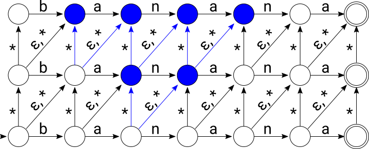
Let’s walk through a simulation of the Levenshtein NFA that accepts all words within edit distance 2 of “banana”. We’ll feed it the input string “bahama”. The set of active states are highlighted in blue at each step below. First, the initial state of the NFA contains all states on the diagonal including the initial state:

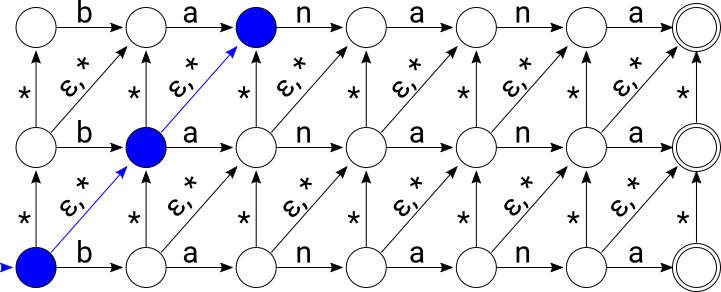
After consuming “b”, active states are again highlighted in blue:

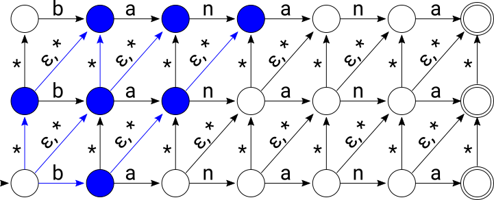
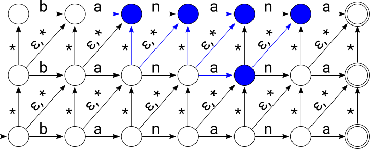
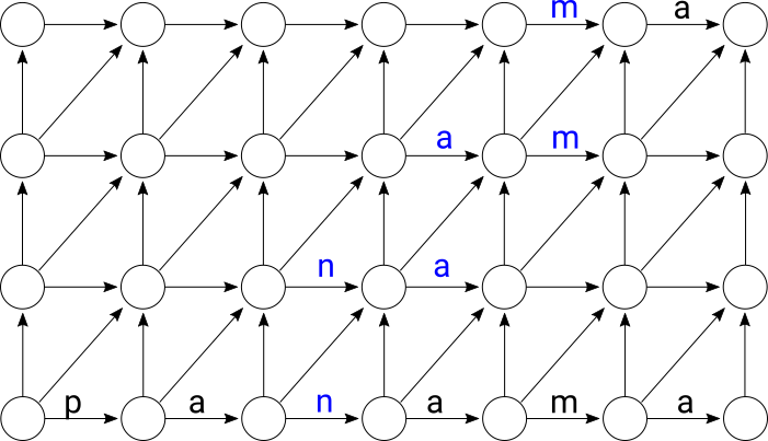
After consuming “ba”:

After consuming “bah”:

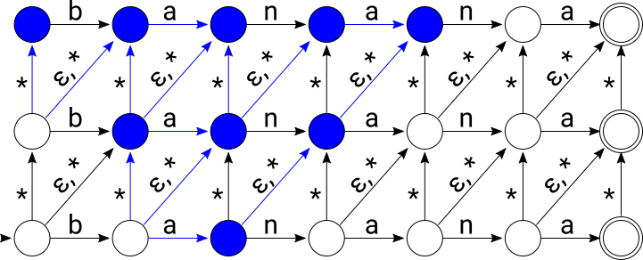
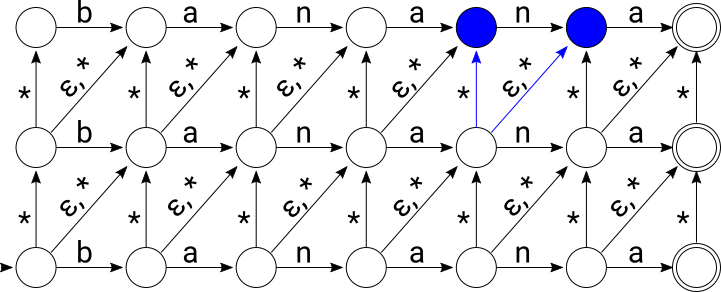
After consuming “baha”:

After consuming “baham”:

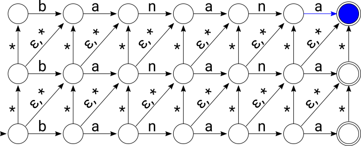
And finally, after consuming “bahama”, a string that’s edit distance 2 from “banana”, we end up in an accepting state:

We want to bound the time complexity of simulating an NFA from this family of Levenshtein NFAs. One way to do this is to bound the maximum number of possible active states, since simulating the NFA on an input of length n involves updating the entire set of active states n times. Since a Levenshtein NFA created for a word of length m and edit distance d has (m + 1) * (d + 1) states, this means that the worst-case time complexity for simulating that NFA on an input of length n could be as bad as O(nmd). We can get a better bound by being a little more careful in our simulation.

The first thing to notice about the family of Levenshtein NFAs is that the diagonals contain paths of epsilon transitions all the way up. This means that any time a state is active, all other states further up on the same diagonal are active. Instead of keeping track of the set of active states, then, we can just keep track of the lowest active state on every diagonal. We’ll call this minimum active index the “floor” of the diagonal.

We’ll start numbering floors from the bottom: any diagonal with a state active in the bottom row of NFA states has floor 0. Since there are d + 1 rows in the NFA, the maximum floor a diagonal can have is d.

To make sure that every state in the NFA is contained in some diagonal, we just need to create a few fake diagonals that extend out to the left a little bit to add to the set of diagonals that are anchored by the states in the bottom level of the NFA:

Indexed like this, a Levenshtein NFA has m + d + 1 diagonals. This means that any active state in the NFA can be represented by a set of at most m + d + 1 diagonal floors.

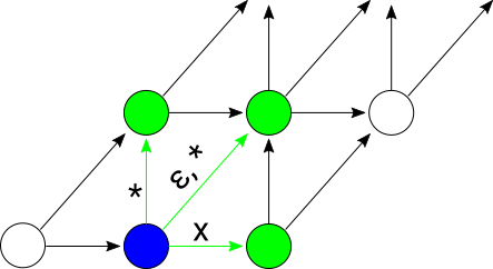
Actually, we never end up needing to consider all m + d + 1 diagonals at once. There’s only ever one diagonal with floor 0 at any point in time, since consuming an input character while one diagonal has a floor at position 0 transfers the state to position 1 in the previous diagonal, position 1 in the current diagonal, and possibly to position 0 in the next diagonal:

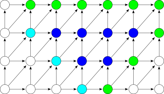
This fact generalizes to higher positions in the set of diagonals: there’s always a sliding window of at most 2d + 1 diagonals that are active at level d or lower. You can prove this by induction on d where the general induction step looks at a window of 2d - 1 diagonals at level d - 1 and shows that they can expand to a window of at most 2d + 1 at level d.

A particular example of the general case is illustrated below, with a starting state illustrated by all light blue and dark blue nodes. These light blue and dark blue nodes cover 5 diagonals at level 2 or lower. The green nodes illustrate all new nodes that can be active after a transition from this state. The green and dark blue nodes together illustrate possible active nodes after the transition, covering 7 diagonals at level 3 or lower:

All of this means that instead of tracking all m + d - 1 diagonals, we only ever need to track a set of 2d + 1 diagonal positions plus an offset into the NFA. The sliding window of diagonals that we track moves through the NFA and we increment the offset by one each time we consume an input character.

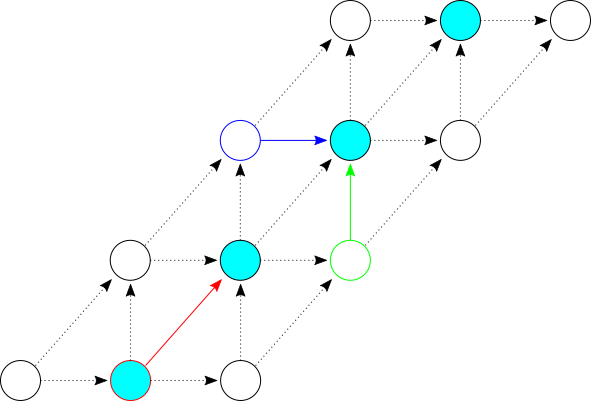
To update a single diagonal when we read an input character, we need to take the minimum of:

• The previous floor of the diagonal, plus one (shown in red below).
• The previous floor of the next diagonal, plus one (shown in green below).
• The smallest index in the previous diagonal that has a transition on the input character, if any (shown in dark blue below).

The figure below shows all three of the contributions to a single diagonal’s update:

Since we’re storing the state as a collection of 2d + 1 diagonal floors plus an offset, the first two items in the list above (red and green updates in the figure above) can be computed in constant time. The third item can be computed by iterating over all d + 1 horizontal transitions from the previous diagonal to see if any match the current input character.

Here’s pseudocode for our current algorithm for a fixed value of d with a few details omitted:

// Returns a structure representing an initial state for a Levenshtein NFA. The
// State structure just contains:
//  * d, the edit distance.
//  * An array of 2*d + 1 integers representing floors.
//  * An integer offset into the underlying string being matched.
State InitialState(d) { ... }

// Returns the floor of the ith diagonal in state s. Returns d + 1 if i is
// out of bounds.
int Floor(State s, int i) { ... }

// Returns the smallest index in the ith diagonal of state s that has a
// transition on character ch. If none exists, returns d + 1.
int SmallestIndexWithTransition(State s, string w, int i, char ch) { ... }

// Set the ith diagonal floor in state s to x.
void SetDiagonal(State* s, int i, int x) { ... }

// Returns true exactly when the given state is an accepting state.
bool IsAccepting(State s) { ... }

// Simulate the Levenshtein NFA for string w and distance d on the string u.
bool SimulateNFA(string w, int d, string u) {
  State s = InitialState(d)
  for each ch in u {
    State t = s
    t.offset = s.offset + 1
    for i from 0 to 2*d + 1 {
      int x = Floor(s, i + 1) + 1                       // Diagonal
      int y = Floor(s, i + 2) + 1                       // Up
      int z = SmallestIndexWithTransition(s, w, i, ch)  // Horizontal
      SetDiagonal(&t, i, Min(x, y, z))
    }
    s = t
  }
  return IsAccepting(s)
}

For each of the n characters in the input string, we iterate over the 2d + 1 diagonals in the state and compute the three components of the diagonal update. Two of the three components (x and y in the pseudocode above) are floor computations which are really just array accesses, so they’re both constant time operations. The third component (z in the pseudocode above, the result of SmallestIndexWithTransition) is the most expensive, taking time O(d) to compute, so the inner loop takes time O(d²) and the entire simulation takes time O(nd²).

An O(nd)-time simulation

To get from O(d²) to O(d) time per state transition and O(nd) for the entire simulation, there’s one final trick: making the SmallestIndexWithTransition function in the pseudocode above run in constant time.

SmallestIndexWithTransition needs to be called on each of the at most 2d + 1 active diagonals to find the smallest index above the floor of the diagonal with a horizontal transition on the current input character. Luckily, there’s a lot of overlap between the horizontal transitions of two consecutive diagonals: if you read the horizontal transitions of any diagonal from bottom to top, they form a substring of length d + 1 of the string the automaton was generated with. Any two consecutive diagonals have an overlap of d characters in these substrings:

The horizontal transitions from a set of 2d + 1 consecutive diagonals span a substring of length at most 3d + 2. This overlap between the horizontal transitions of consecutive diagonals means that instead of iterating up each diagonal doing O(d) work to figure out the first applicable horizontal transition, if any, for each of the 2d + 1 diagonals, we can instead precompute all the transitions on the substring of length 3d + 2 once and use that precomputed result to calculate SmallestIndexWithTransition on each diagonal.

This precomputation just involves calculating, for each index in the 3d + 2 character window, the next index in the window that matches the current input character. For example, if the window was the string “cookbook”:

    [c][o][o][k][b][o][o][k]
     0  1  2  3  4  5  6  7

our precomputed jump array for the character ‘k’ would look like:

    [3][3][3][3][7][7][7][7]
     0  1  2  3  4  5  6  7

Each index in the jump array tells us the next index of the character ‘k’ in the window. If we look in the jump array at the index of a particular diagonal plus its floor, the jump array tells us the next applicable horizontal transition on that diagonal.

The jump array needs to be initialized once per transition but initialization only takes time O(d) and all subsequent calls to SmallestIndexWithTransition can then be implemented with just a constant-time access into the jump array. Now everything inside the for loop that iterates over 2d + 1 diagonals runs in constant time and computing a transition of the NFA only takes time O(d).

Final Thoughts

I’ve implemented all of this in the Go package levtrie and the code in that package is a better place to look if you’re interested in more details after reading this post.

I took some shortcuts there to make the code a little more readable at the expense of some unnecessary memory bloat. In particular, the Trie implementation is very simple: each node keeps a map of runes to children and no intermediate nodes are suppressed. The key for each node, implicitly defined by the path through the Trie, is duplicated in the key-value struct stored at each node.

If you’re looking to implement something similar and speed it up, the first thing to consider is replacing the basic Trie with a Radix or Crit-bit tree. A Crit-bit tree will dramatically reduce the memory usage and the number of node accesses needed for Trie traversals, but it will also complicate the logic of the parallel search through the Trie and Levenshtein Automaton. Instead of iterating over all runes emanating from a node in the Trie and matching those up with transitions in the Levenshtein Automata, you’ll have to do something more careful. You could add some logic to traverse the Crit-bit tree from a node, simulating an iteration over all single-character transitions. Multi-byte characters make this a little more tricky than an ASCII alphabet. You might have an easier time converting the the Levenshtein Automata itself to have an alphabet of bytes instead of multibyte characters, which would then match up better with a Radix tree with byte transitions.